How to Create a Dynamic Excel Chart
This post is a how-to guide for creating a dynamic Excel chart. When I say dynamic, I mean that there will be a drop down list in which you can choose the variable you would like to display, and the chart will automatically graph the data. This chart will be helpful for anybody who needs to quickly graph data for experimental or presentation purposes. I personally use charts like this often in lab meeting or project update presentations. This one chart saves me time from having to create multiple Excel charts for projects in which I have hundreds of variables to view.
This guide is written with the assumption that the reader has a basic understanding of Excel and how to write equations in cells. If you are completely clueless about Excel, you’ll still be able to create a chart, but it just may take a little longer to figure out some of the steps. I have tried to add as many pictures as possible to give you an idea of what each step will look like as you go along.

Activate Developer Tab
First things first, you need to activate the Developer tab. The Developer tab allows you to add all kinds of cool options to an Excel sheet, but the only Developer option we will use today is the Combo List. To activate the Developer tab, you will need to go to File (located at the top left of the sheet) and choose Options. A box with Excel options will pop up and you will need to select Custom Ribbon (located on the left about halfway down). After choosing Custom Ribbon, the right side of the box will show all of the tabs available, and you need to make sure that the Developer box is checked. Once checked, hit OK and we’re off to the races.

Name Your Sheets
At the bottom of you Excel sheet there will be a tab with the name of the sheet (typically Sheet 1 by default). If only one tab is visible you will need to add another by hitting the + button. Once you have the two tabs, rename the first one “Data” and the second one “Chart” by right-clicking on the tab and selecting “rename”.

Create Data Sheet
Make sure you have the Data sheet selected, and then manually type in a vertical list of variables and a horizontal list of samples as shown in the picture. For this guide, I have chosen 7 variables (A-G) and 10 samples (1-10). If you want to be fancy, you can add in formatting by outlining the cells and making the font bold, but this is not needed for the chart to be functional. This sheet is where the data you want to be graph will be pulled from.

Insert Chart
Now switch over to the “Chart” tab by selecting the correct tab at the bottom of the page. Once the Chart tab is selected, go up to the top of the page and select the Insert tab. Click the Column button, and choose the first 2-d column chart. A blank chart will automatically be added to the sheet. Move this rectangle up to the top left of the sheet. You will be able to resize it later on if needed.
Pull Data from Data Sheet
Still working on the Chart tab, you need to go to Column B and Row 18. In this cell, type “=Data!B11”. This equation copies the data from the Data sheet. If you have followed along correctly, this cell should now display “Variables” after you hit enter. You want to copy this procedure by copying this cell and pasting it into the location below and to the side of B:18. You sheet should now look like the picture below.

Name Your Data
So that your chart will know how to graph your data, you will need to name your data. To do this, go to the top of the page and click the Formulas tab. Next, select Name Manager. A box will pop up and you will need to enter “dataset” into the name box. To designate what it refers to, click on the box located to the right of “Refers to” and then highlight all of the cells that currently contain 0’s.

Insert Drop-down List (Combo Box)
Now comes the fun. Head up to the top of the sheet and click on the Developer tab. Next, click on the Insert button. Selected the second icon (called Combo Box). Now select where you want the list to be located. In the example I clicked on cell J:2. A square button with a triangle will appear. I would recommend resizing the rectangle similar to what is seen in the picture below.

To be able to add your variables (A-G) to the drop-down list, you need to right-click on the drop-down list and select “format control”. In the “input range” box, highlight your variables cells B:19 through B:25.
Next, in the “Cell link” box, you want to enter “$I$2”. Now, if everything is working correctly, a number will appear in cell I:2 that corresponds to whichever variable you choose. For example, if you select “A” the number 1 will appear. Likewise, if you select “G”, the number 7 will appear.
Designating the Results
For the chart to select the right data to graph, we need to set up an equation that will find the correct data that corresponds to the variable you choose. To begin, I typed “Results” into cell B:16 so that I would know where my results would be located. Next, in cell C:16, you need to write “=INDEX(dataset,$I$2,C$17)”. Next copy and paste this into the next 9 cells to the right.

Setting up the Chart
Right-click on the chart area and choose “Select Data”. Select “Add” and a second box will appear. Click in the box and enter “1”. Next, click in the “Series values” box and then highlight cell C:16.

Repeat this step to add the rest of your samples (2-10). For each sample, enter the following:
Sample 2 – enter “=Chart!$D$16”
Sample 3– enter “=Chart!$E$16”
Sample 4– enter “=Chart!$F$16”
Sample 5– enter “=Chart!$G$16”
Sample 6– enter “=Chart!$H$16”
Sample 7– enter “=Chart!$I16”
Sample 8– enter “=Chart!$J$16”
Sample 9– enter “=Chart!$K$16”
Sample 10– enter “=Chart!$L$16”
Your excel sheet is now ready to rock and roll!
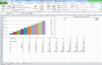
To test it out, go back to your Data tab at the bottom of the sheet. Enter random values in all of the boxes.
Now go back to your Chart tab and see if the values are graph like they are supposed to be. If you find that something is not working correctly, you may need to make sure there are no misspelled equations.
If you have questions or suggestions, feel free to comment below.